

What an LLM is trying to do
An LLM is, at its core, trying to build a statistical model of the language data it was trained on. The cleanest way to imagine what this means is to picture yourself in a familiar place: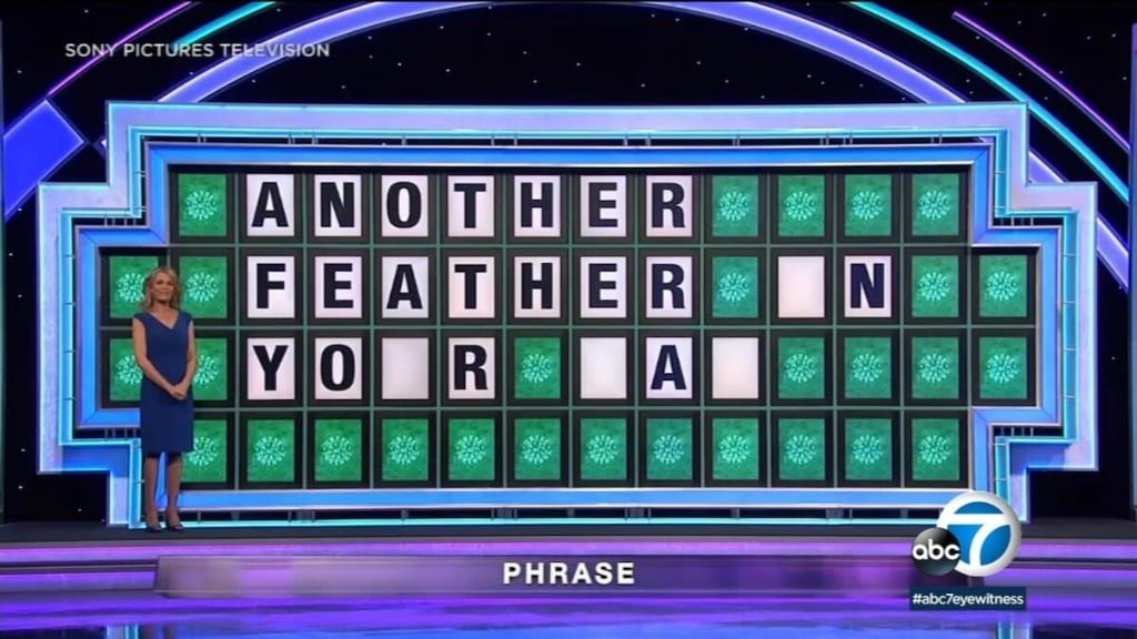
Calling an LLM API
Here is about the simplest call you can make on Together AI. We hand a text model the start of a sentence and ask it to continue, capped at a single token of output:"The largest city in France is" turns into something like:
max_tokens=1, the inference engine takes the single most likely index, decodes it back to text, and hands you " Paris". (In practice, you might need more than one token to reliably finish the sentence.)
To produce a longer reply, the inference engine repeats these steps in a loop:
- Convert the current input into a list of integer indices (token IDs).
- Run the model on the current input.
- Look at the probabilities for the next token.
- Pick the next token.
- Add it to the end of the input.
- Repeat until the model produces a stop signal or you hit a length limit.
Text becomes tokens, tokens become vectors
When the model receives your input text, it first converts it into a list of token IDs (integer indices). After that, it turns each ID into a vector or embedding: a list of floats, typically 1,024 to 16,384 long. The model has a learned lookup table that maps each token ID to a vector. That vector is the model’s working representation of the token, or its “embedding”. Why is each token represented as a vector? Two reasons:- First, you can’t do useful math on raw token IDs, ID 5279 and ID 5280 are arbitrary. With vectors, the model can express that “Paris” and “Lyon” are similar in some directions and different in others, literally by placing their vectors close together along the “city” axis and far apart along the “size” axis.
- Second, the main operation throughout the model is a matrix multiplication (matmul): you multiply a vector by a matrix (a grid of numbers) to get a new, transformed vector, and that only works on vectors, not raw integer IDs. The numbers filling those matrices are the model’s weights, so a learned matrix (a term that comes up later) just means one of these grids, with values found by training rather than set by hand.
The transformer block
After the embedding step, every token is a vector, but that vector still only reflects the token in isolation. The embedding for “bank” is identical whether the sentence is “river bank” or “savings bank.” The job of the transformer is to refine each vector until it captures what the token means in this particular context. It does that by passing the vectors through N identical layers (blocks), where N is usually between 32 (small models) and 120+ (frontier models). Every block runs the same two steps:- Attention: Each token gathers information from the earlier tokens in the sequence and folds the relevant parts into its own vector. This is the only step where tokens exchange information.
- Feed-forward network (FFN/MLP): Each token’s vector is then processed on its own, with no reference to the others. This is where the model applies the knowledge stored in its weights to the now-contextualized vector.
Attention
For each token, the attention step computes three things from the token’s current vector by multiplying it with three different learned matrices:- A query (Q), “what am I looking for?”
- A key (K), “what do I look like to others?”
- A value (V), “what do I have to share?”
- Causal mask: A token at position 5 can only look at positions 0-4. Never the future. That’s what makes the model autoregressive: At training time, it can’t peek at the next word it’s supposed to predict, and at inference time, it can’t look at tokens that haven’t been generated yet.
- Multi-head: This whole process runs in parallel many times (typically 32-96 “heads”), with different learned matrices each. Different heads end up specializing in different patterns—one might track the most recent noun, another might find matching brackets in code, another the subject of the current clause.
- Q, K, and V are learned matrices: The interpretation of Q, K, and V above is a useful analogy for explaining what attention does, but in practice it’s all matrix multiplication. The model figures out what to put in those matrices during training, purely from the process of trying to predict the next word.
Feed forward network (FFN)
After attention has mixed information across tokens, the feed forward network (FFN) (AKA multilayer perceptron, or MLP) processes each token’s vector on its own. It widens the vector (typically to 4× its size) by multiplying it with one matrix, applies a nonlinear function, then narrows it back down with another matrix. This is where most of the parameters in the model actually live. By raw count, the feed forward network layers dwarf the attention layers. A useful way to think about it is that this is where the model stores all of its knowledge about the world. The widening step is like asking many questions about the token’s current state in parallel, while the narrowing step writes back the answers. Most of the model’s “world knowledge”—what cities are capitals, which functions Python has, that one programming language uses curly braces and another uses indentation—is stored in the feed forward network weights. Nobody has a clean understanding of which weight stores what exactly, because the patterns are distributed across millions of neurons in ways no one fully understands. The entire field of interpretability is trying to answer exactly this question.Picking a token
After the last block, each position holds a vector that summarizes everything the model thinks up to that point. To turn this into a prediction for the next token, one final linear layer projects the vector back to the vocabulary, producing one number for each possible next token. These numbers are called logits. Logits are raw scores, not probabilities, and they can be any real number, including negative ones. To turn them into probabilities, you apply a softmax operation: exponentiate each logit and normalize. This ensures that the probabilities are all positive and sum to 1 (which is a requirement for a valid probability distribution). Then you pick / sample a token. The most basic choice is to pick the highest-probability token (greedy decoding), but several controls—temperature, top-k, and top-p—shape the distribution before sampling. See inference parameters & sampling for more details.What training actually does
Everything covered above—the matmuls, the attention, the FFN / MLPs, the softmax—is fixed and constant. The model’s behavior comes from the numbers inside those matrices. Those numbers are called weights. They start off random, and during the training process, the model searches for useful values for each weight. This process of taking the weights from random initializations to useful values is called pretraining, and it costs millions of dollars in compute, can take months to complete. Pretraining works like this:- Take a document from the training data (anything from Wikipedia to GitHub to chat logs).
- For every position in that document, ask the model what comes next.
- Compare its prediction to the actual next token. The mismatch between the prediction and the actual next token is called the loss.
- Compute how much each weight contributed to the loss.
- Nudge each weight a tiny bit in the direction that would have reduced the loss. This is called backpropagation.
- Instruction tuning: Training the pretrained model on examples of “good behavior” (helpful answers, polite refusals, structured output) so it stops continuing text and starts responding to instructions.
- Preference tuning: Approaches like reinforcement learning from human feedback (RLHF) and direct preference optimization (DPO) run a feedback loop where pairs of “good” and “bad” outputs nudge the model toward outputs people actually want.
- Reinforcement learning with verifiable rewards (RLVR): Training on tasks whose answers can be checked automatically (math problems, code that passes tests, puzzles with a known solution), so the model gets rewarded for actually being right rather than for sounding right. This is the trick behind modern “reasoning” models that think out loud before answering.
Next steps
Tokens & tokenization
What happens to the input text before the model sees it.
Context windows
How much input the model can take in a single request (and why there’s a hard limit).
Inference parameters & sampling
Available controls for shaping the output.